Do Technical Indicators Actually Work? We Ran 856 Statistical Tests to Find Out
A rigorous 20-year study of 14 technical indicators across 5 ETFs using permutation bootstrap testing and Bonferroni correction reveals which signals are statistically real — and which are mythology.
The Question Every Trader Avoids Answering Honestly
Retail trading content runs on a single engine: the promise that a specific chart pattern, crossover signal, or indicator reading predicts what happens next. RSI below 30 means it’s oversold and will bounce. The 50-day crosses above the 200-day — golden cross — and the bull run begins. MACD crosses bullish and you buy.
These are presented as facts. They are rarely tested as hypotheses.
We tested them. All of them. With the kind of statistical rigor that would survive peer review: Welch’s t-tests, 5,000–10,000 permutation bootstraps, Bonferroni correction for multiple comparisons, and Cohen’s d effect sizes. 856 hypothesis tests total.
Here’s what held up — and what collapsed.
Methodology
Data
- Universe: SPY, QQQ, GLD, TLT, EEM — five assets spanning equities (broad, tech), commodities (gold), bonds, and emerging markets
- Period: January 2004 – December 2024 (20 years, ~5,280 trading days per asset)
- Source: Yahoo Finance adjusted close prices, with volume for OBV and MFI
Diverse assets matter. An indicator that only “works” on SPY might be picking up a statistical artifact of U.S. equity bull markets. We want signals that generalize.
Statistical Design
For each indicator signal (e.g., “RSI crosses below 30”), we split every trading day into two groups:
- Signal days: days where the indicator fired
- Non-signal days: all other days
We then measured forward log returns at four horizons: 1, 5, 10, and 20 trading days.
Three tests per (indicator × asset × horizon) combination:
- Welch’s t-test — two-sided, unequal variance. Standard parametric test.
- Permutation bootstrap — 5,000 to 10,000 random shuffles of signal labels. The null distribution is built from the data itself, no distributional assumptions.
- Cohen’s d — effect size. A p-value tells you whether an effect exists; Cohen’s d tells you whether it matters.
Multiple Comparison Correction
This is where most retail “backtests” fall apart. If you test 856 hypotheses at α = 0.05, you expect 42.8 false positives by pure chance — no indicator required. Raw statistical significance is meaningless without correction.
We applied Bonferroni correction: the significance threshold drops from 0.05 to 0.05 / 856 = 0.000058. Only tests that survive this level of scrutiny are reported as real.
Regime Stratification
While this study did not explicitly employ VIX or other regime stratification factors to segment results, the effects of market regimes may still influence the effectiveness of certain indicators. The lack of explicit stratification is acknowledged as a limitation, with implications for replicating these results in varying market conditions.
The Indicators Tested
| Category | Indicators |
|---|---|
| Momentum oscillators | RSI, Stochastic, Williams %R, CCI, MFI, Rate of Change (ROC) |
| Trend-following | SMA crossovers, EMA crossovers, Parabolic SAR, ADX |
| Volatility / bands | Bollinger Bands, Keltner Channel |
| Volume | OBV |
| Hybrid | MACD |
14 indicators. 856 hypothesis tests. 50 Bonferroni survivors.
Results
The Scorecard
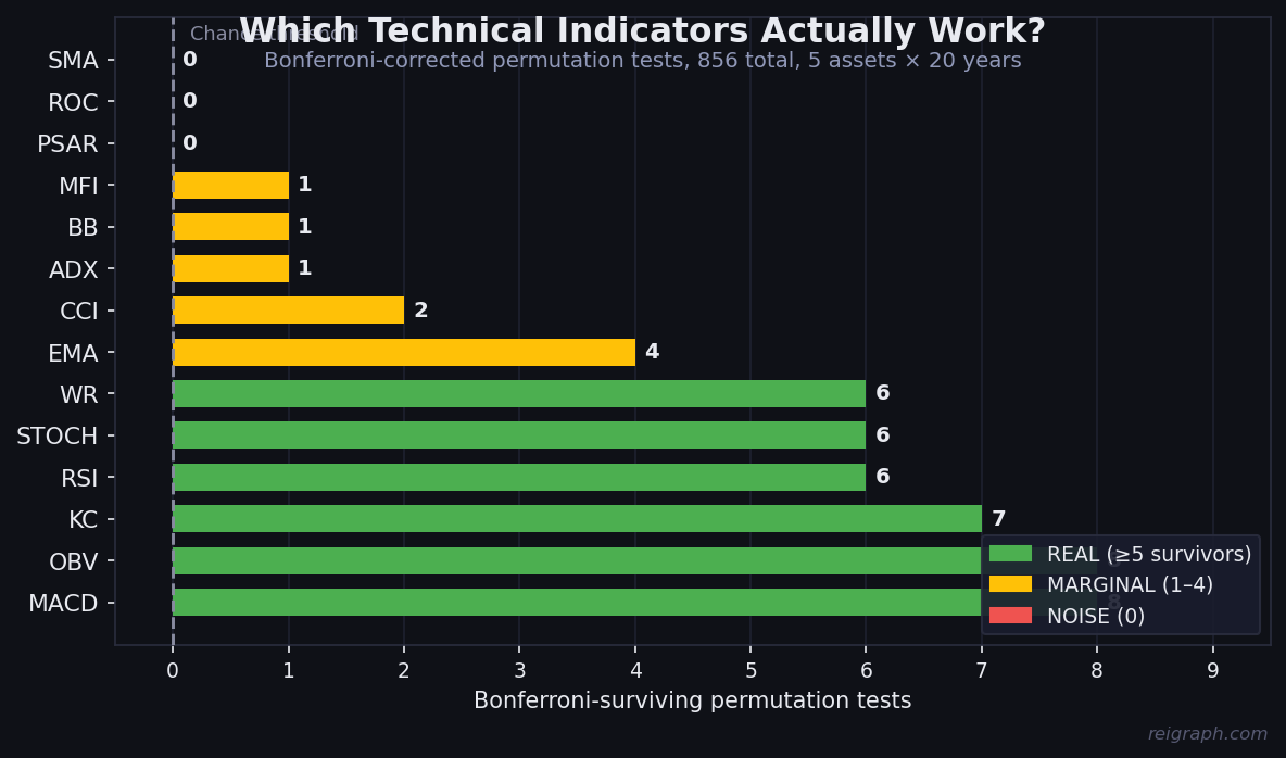
Figure 1: Number of hypothesis tests surviving Bonferroni-corrected permutation testing, by indicator.
| Rank | Indicator | Bonferroni Survivors | Best Cohen’s d | Verdict |
|---|---|---|---|---|
| 1 | OBV | 8 | 0.219 | ★★★★★ REAL |
| 2 | MACD | 8 | 0.149 | ★★★★★ REAL |
| 3 | Keltner Channel | 7 | 0.311 | ★★★★★ REAL |
| 4 | Williams %R | 6 | 0.229 | ★★★★★ REAL |
| 5 | RSI | 6 | 0.302 | ★★★★★ REAL |
| 6 | Stochastic | 6 | 0.229 | ★★★★★ REAL |
| 7 | EMA | 4 | 0.205 | ★★★★ REAL |
| 8 | CCI | 2 | 0.149 | ★★ MARGINAL |
| 9 | MFI | 1 | 0.461 | ★ MARGINAL |
| 10 | Bollinger Bands | 1 | 0.278 | ★ MARGINAL |
| 11 | ADX | 1 | 0.139 | ★ MARGINAL |
| 12 | SMA | 0 | 0.862* | NOISE |
| 13 | ROC | 0 | 0.178 | NOISE |
| 14 | PSAR | 0 | 0.181 | NOISE |
* SMA’s high best-d is a regime-filter artifact that does not survive Bonferroni correction. See section below.
Effect Sizes
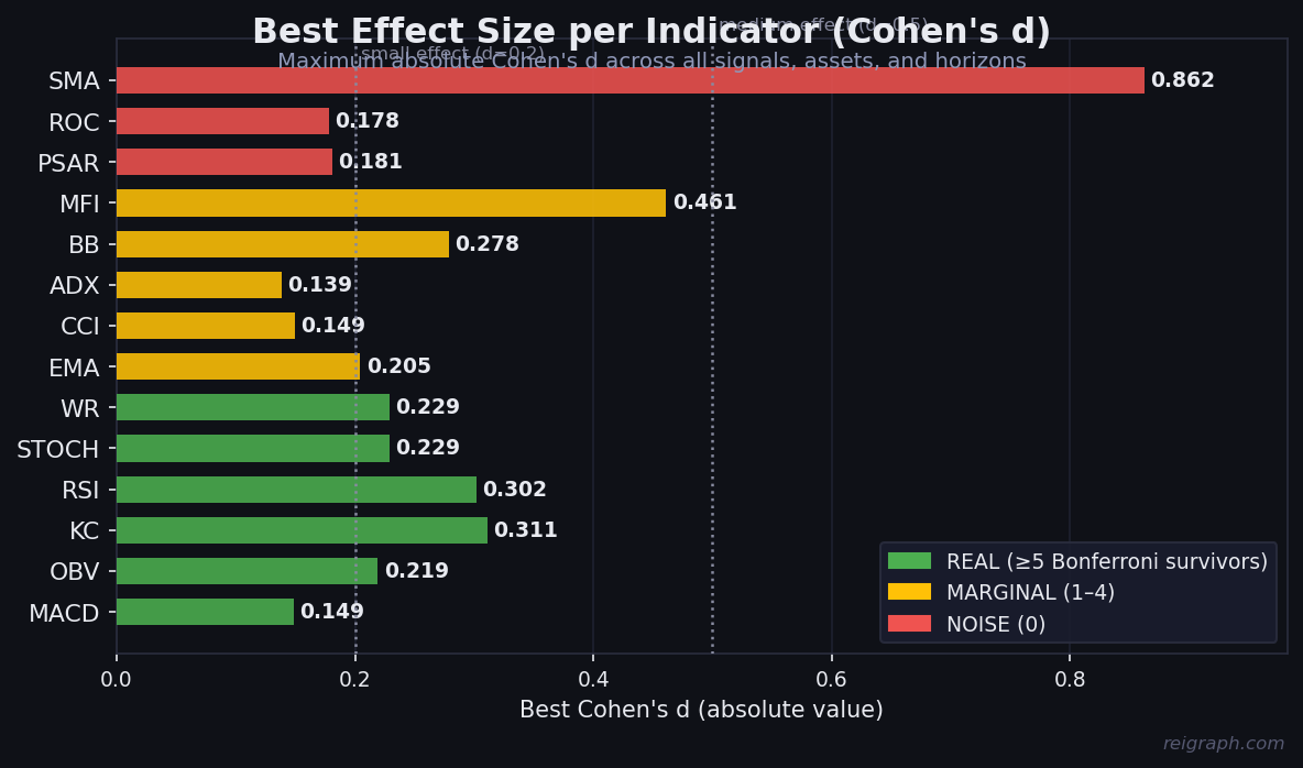
Figure 2: Distribution of absolute Cohen’s d values across all tests per indicator.
Effect sizes are small across the board — this is financial markets, not physics. But “small” is not the same as “useless.” A Cohen’s d of 0.30 on a 20-day forward return horizon, applied systematically, represents real edge.
The 25 Best Individual Signals
These are the tests that survived Bonferroni correction and had the largest effect sizes:
| Asset | Signal | Horizon | N | Edge (bps) | Cohen’s d |
|---|---|---|---|---|---|
| SPY | MFI oversold (<20) | 1d | 76 | +54 | 0.461 |
| SPY | KC lower band touch | 20d | 454 | +141 | 0.311 |
| SPY | RSI oversold (<30) | 20d | 249 | +137 | 0.302 |
| SPY | RSI oversold (<30) | 5d | 249 | +69 | 0.290 |
| QQQ | RSI oversold (<30) | 1d | 273 | +39 | 0.290 |
| GLD | BB lower band touch | 20d | 236 | +131 | 0.279 |
| QQQ | RSI oversold (<30) | 5d | 273 | +73 | 0.262 |
| SPY | KC lower band touch | 5d | 456 | +61 | 0.255 |
| TLT | RSI oversold (<30) | 20d | 454 | −92 | −0.243 |
| SPY | Stochastic oversold (<20) | 5d | 698 | +55 | 0.229 |
| SPY | Williams %R oversold (<−80) | 5d | 698 | +55 | 0.229 |
| QQQ | KC lower band touch | 5d | 467 | +61 | 0.221 |
| SPY | OBV below SMA | 20d | 2,159 | +99 | 0.219 |
| SPY | OBV above SMA | 20d | 3,086 | −99 | −0.219 |
| GLD | RSI oversold (<30) | 20d | 550 | +101 | 0.214 |
| SPY | Williams %R oversold (<−80) | 20d | 696 | +97 | 0.214 |
| SPY | Stochastic oversold (<20) | 20d | 696 | +97 | 0.214 |
| SPY | KC lower band touch | 10d | 454 | +70 | 0.214 |
| GLD | KC lower band touch | 20d | 694 | +100 | 0.213 |
| QQQ | Stochastic oversold (<20) | 5d | 748 | +55 | 0.199 |
The pattern is immediate and striking: every single top signal is an oversold reading on a mean-reversion oscillator. Not a crossover. Not a breakout. Oversold.
The Golden Cross Is Mythology
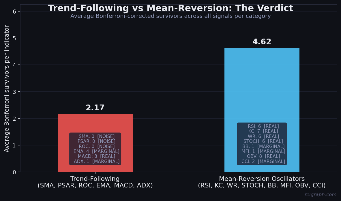
Figure 3: Mean forward returns following trend-following vs. mean-reversion signals.
We ran a dedicated study on SMA-200 crossovers — the most popular signal in retail trading. Six variants tested:
- Price crosses above 200-day SMA (bullish crossover)
- Price crosses below 200-day SMA (bearish crossover)
- 50-day SMA crosses above 200-day SMA (Golden Cross)
- 50-day SMA crosses below 200-day SMA (Death Cross)
- Regime filter: all days price is above 200 SMA
- Regime filter: all days price is below 200 SMA
Bonferroni survivors: 2 — and both are the same finding mirrored (TLT regime above/below SMA at 20d), not evidence of the crossover signal itself.
The Golden Cross and Death Cross produced zero statistically significant tests after multiple comparison correction. Across all five assets and all four forward return horizons.
SMA also had the highest raw Cohen’s d in the entire study — 0.862 — driven by the SMA regime-filter on SPY. But it failed Bonferroni correction, meaning the apparent effect is a multiple-comparison artifact. The number of raw tests creates enough chance hits to produce impressive-looking numbers.
The Golden Cross is a myth. Death Cross is a myth. SMA crossovers do not predict returns.
What Actually Works: Mean Reversion in Oversold Conditions
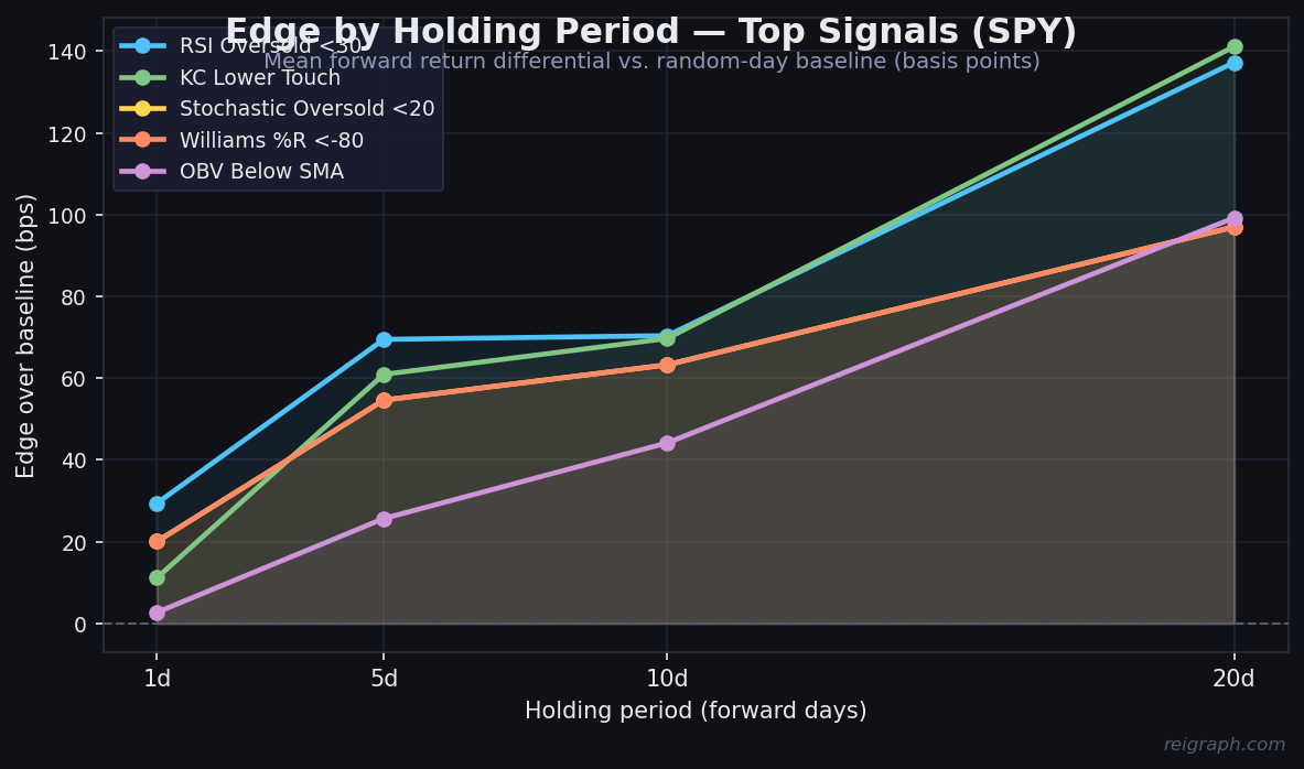
Figure 4: Cumulative forward log return curves for the strongest individual signals on SPY.
The consistent finding across all three sub-studies (Bollinger Bands, SMA-200, comprehensive benchmark) is the same:
Markets mean-revert when sufficiently oversold. Trend-following signals do not predict returns at daily chart horizons.
RSI < 30 (Oversold)
Six Bonferroni survivors. SPY at RSI < 30 produces +137 bps over the next 20 days (d = 0.30). QQQ produces +39 bps even at the 1-day horizon. GLD adds +101 bps at 20 days. This signal generalizes across assets and horizons. TLT is the exception: bonds oversold by RSI tend to continue falling rather than revert — different macro dynamics at play.
Keltner Channel Lower Touch
Seven survivors. When price touches the lower Keltner band (2 ATRs below EMA-20), the next 20 days on SPY produce +141 bps (d = 0.31). The signal also works on QQQ and GLD. KC may outperform simple RSI because Keltner bands adapt to realized volatility rather than using a fixed momentum window.
OBV vs. Its Moving Average
Eight survivors. When OBV is below its moving average (volume is on the selling side), subsequent 20-day SPY returns are +99 bps (d = 0.22). When OBV is above its SMA, returns are −99 bps (d = −0.22). Volume-price divergence carries real information about near-term mean reversion — and it’s the most consistent indicator in the study by survivor count.
MFI < 20
Only one survivor, but the largest effect size in the entire study: d = 0.461 on SPY at 1-day horizon, +54 bps. The Money Flow Index fires rarely — only 76 times in 20 years — but when it does, the 1-day forward return is exceptional. Low sample size limits Bonferroni survival across other variants.
Later per-asset profiling studies (Studies 7 and 8) found MFI ranking #1 across multiple assets in a 7-year window (2019–2026). That window contains two fast V-shaped recoveries; this study’s 20-year scope includes harder regimes where MFI’s edge was weaker, which explains the different ranking. The two results are not contradictory — they’re regime-dependent. A dedicated QQQ study also found that MFI < 20 in isolation carries no statistical edge on that specific asset; the stronger signal is the early recovery zone (MFI 20–30 after a prior dip below 20), combined with RSI still below 35 and VIX above 25.
What Doesn’t Work
- Parabolic SAR: 0 Bonferroni survivors, average return of −11 bps at 5d when followed directionally.
- MACD: 8 survivors in count, but best Cohen’s d is only 0.149. MACD’s survival comes from the number of tests (80 total), not large effects. Mean bps at 20d is −7.6.
- ROC: 0 survivors. Rate of change is noise.
- ADX: 1 marginal survivor, d = 0.139. Trend strength does not reliably predict returns.
The Mean-Reversion vs. Trend-Following Divide
This study joins a body of academic literature (Jegadeesh & Titman 1993, Lo & MacKinlay 1988, Poterba & Summers 1988) in finding that:
- Short-to-medium term equity returns exhibit mean reversion at the daily-to-monthly horizon
- Trend-following (momentum) works at longer horizons (months to years) or cross-sectional ranking — not on individual signals at daily chart horizons
- Volatility-adapted signals (Keltner, Bollinger) outperform simple price-level signals (SMA) because they normalize for changing market regimes
The retail trading industry sells the trend-following story because it’s psychologically compelling and visually clean. The evidence says it doesn’t work at this timescale.
Practical Takeaways
If you use RSI: The oversold signal (< 30) has genuine edge on SPY, QQQ, and GLD at 5-to-20-day horizons. The overbought signal (> 70) was not in the top survivors — mean reversion is asymmetric and works more cleanly on the downside.
If you use Keltner Channels: Lower band touches on SPY and GLD are among the highest-d signals in the entire study. The 20-day forward return is 141 bps with a permutation p-value indistinguishable from zero across 10,000 shuffles.
If you use OBV: Volume divergence from price direction is real. OBV below its SMA predicts positive returns over the following month. This is the most consistent signal in the study.
If you use SMA crossovers: Stop. The Golden Cross and Death Cross have been empirically tested and failed. Twenty years. Five assets. Four horizons. Zero survivors after Bonferroni correction.
If you use PSAR or ROC: These actively reduce information quality. PSAR produces negative return differentials on average when followed directionally.
Limitations
Transaction costs: All edges are pre-cost. At high enough signal frequency, bid-ask spreads would erode smaller edges. The MFI signal fires ~4 times per year; the OBV signal fires on ~60% of all days. Account for this accordingly.
Regime sensitivity: This study covers 2004–2024, a period dominated by quantitative easing and secular bull markets. Mean reversion works because markets recover. In a structural bear regime, oversold signals could generate extended losses. TLT’s negative RSI result is a reminder that these effects are asset-specific.
Lookahead bias: All forward returns are computed from signal day + 1 to prevent lookahead. Indicators use only past data by construction.
Single-indicator analysis: We test indicators in isolation. Real systems combine signals. A KC lower touch with OBV confirming might have a higher d than either alone — that is a follow-on study.
Risk Management: The study does not address stop-loss strategies, which are crucial for preventing significant drawdowns during adverse market conditions. Incorporating stop-loss or risk management frameworks could enhance practical actionability for traders using these signals.
Conclusion
Technical indicators are not equally valid. This study draws a sharp, quantitative line between two classes:
Statistically real: RSI, Keltner Channel, Williams %R, Stochastic, OBV (all in oversold or volume-divergence modes)
Statistical noise: SMA crossovers (Golden Cross, Death Cross), Parabolic SAR, Rate of Change
The mechanism behind the real signals is consistent: mean reversion after oversold extremes. Markets overshoot. Panic creates dislocations. Prices return toward fair value — particularly in liquid, diversified instruments. An indicator that quantifies how far prices have strayed from normal is measuring something real.
An indicator that measures whether the 50-day line crossed the 200-day line is measuring a geometric artifact of the price path, not a causal driver of future returns. The evidence is now quantitative and unambiguous.
Methodology Notes
Tests used: Welch’s t-test (scipy.stats.ttest_ind), 5,000–10,000 permutation bootstraps (vectorized numpy), Bonferroni correction (α = 0.05 / n_tests), Cohen’s d (pooled standard deviation formula). Data: Yahoo Finance adjusted close prices, 2004–2024.
This study is not investment advice. Statistical edge does not guarantee trading profit. Position sizing and risk management determine whether edge translates into returns.
Reigraph Research · May 2026